This notebook can be found on github

Gaussian wave packet running into a potential barrier

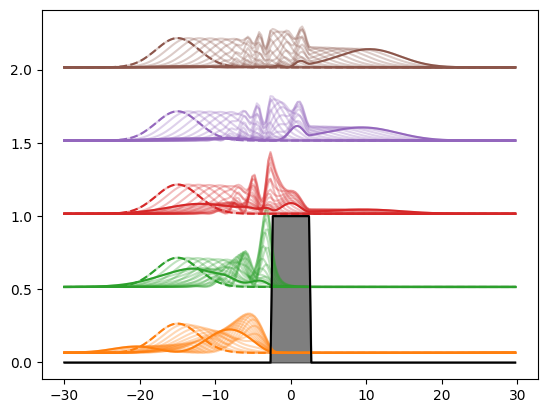
In this example, we simulate the dynamics of a Gaussian wave packet that runs into a square potential barrier. In this, we make use of the FFT relations between position and momentum bases, which allows us to boost the efficiency of the calculation. To this end, the so-called Lazy operatorations (LazyProduct and LazySum) are used.

using QuantumOptics
using PyPlot

First, we define a position basis and calculate the respective momentum basis by means of an FFT (numerically by simply passing the position basis as argument). The position basis is defined by its range in space.

xmin = -30
xmax = 30
Npoints = 200

b_position = PositionBasis(xmin, xmax, Npoints)
b_momentum = MomentumBasis(b_position)

Once this is done, we define a sqaure potential barrier of width $d$ and height $V_0$ in the position basis.

V0 = 1. # Height of Barrier
d = 5 # Width of Barrier
function V_barrier(x)
    if x < -d/2 || x > d/2
        return 0.
    else
        return V0
    end
end
V = potentialoperator(b_position, V_barrier)

For the kinetic energy term we can exploit that it is diagonal in the momentum basis. In the time evolution we want to first transform the density operator from the position to the momentum basis, multiply it with the kinetic operator and then transform it back. This can be done by using the FFTOperator which when applied to a density operator will perform such a transformation. The LazyProduct operator makes it possible to chain these three operations together.

Txp = transform(b_position, b_momentum)
Tpx = transform(b_momentum, b_position)
Hkin = LazyProduct(Txp, momentum(b_momentum)^2/2, Tpx)

Since the kinetic energy operator is never really calculated and only its action onto a density operator is defined we also cannot directly add another operator to it. Instead we also have to delay this sum so that it is only performed indirectly when applied to a density oeprator. This can be done with the LazySum operator.

H = LazySum(Hkin, V)

Finally we let gaussian wave packets start on the left side of the barrier and analyze the time evolution. The offset of the packet on the y-axis here indicates the initial kinetic energy.

xpoints = samplepoints(b_position)

x0 = -15
sigma0 = 4
p0vec = [sqrt(0.1), 1, sqrt(2), sqrt(3), 2]
timecuts = 20

for i_p in 1:length(p0vec)
    p0 = p0vec[i_p]
    Ψ₀ = gaussianstate(b_position, x0, p0, sigma0)
    scaling = 1.0/maximum(abs.(Ψ₀.data))^2/5
    n0 = abs.(Ψ₀.data).^2 .* scaling

    tmax = 2*abs(x0)/(p0+0.2)
    T = collect(range(0.0, stop=tmax, length=timecuts))
    tout, Ψt = timeevolution.schroedinger(T, Ψ₀, H);

    offset = real.(expect(Hkin, Ψ₀))
    plot(xpoints, n0.+offset, "C$i_p--")
    for i=1:length(T)
        Ψ = Ψt[i]
        n = abs.(Ψ.data).^2 .* scaling
        plot(xpoints, n.+offset, "C$i_p", alpha=0.3)
    end
    nt = abs.(Ψt[timecuts].data).^2*scaling
    plot(xpoints, nt.+offset, "C$i_p")
end
y = V_barrier.(xpoints)
fill_between(xpoints, 0, y, color="k", alpha=0.5);
plot(xpoints, y, "k")